How to Cross Out Text in Excel Using Strikethrough

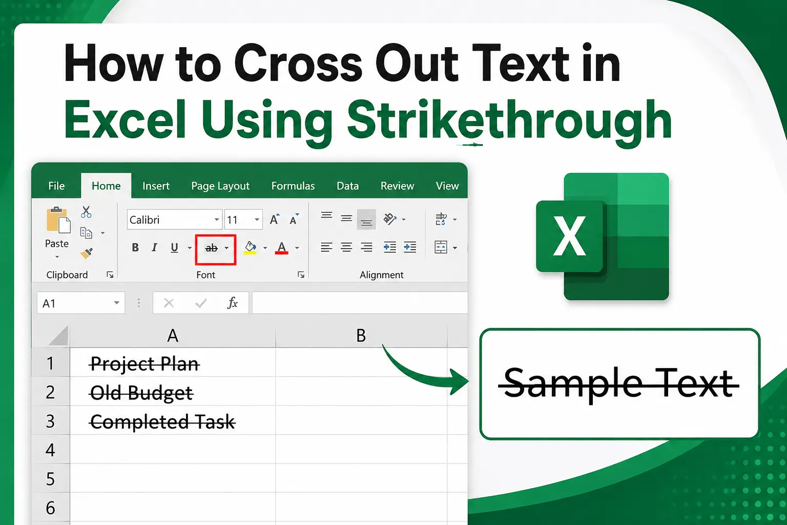
Excel is used for many things beyond simple numbers. People use it for to-do lists, project trackers, and daily task sheets. One common need in these spreadsheets is marking something as finished or outdated.

This is where strikethrough formatting comes in. It lets you cross out text in Excel without deleting it completely. The information stays visible, but it’s clearly marked as done or no longer relevant.

In this guide, Teche Advice explains every method to cross out text in Excel. We keep things simple, using short sentences and clear steps. By the end, you will know several easy ways to apply this formatting, whether you prefer shortcuts, menus, or automatic rules.

Let’s get started.

Crossing out text simply means adding a line through the middle of your text. This formatting style is called strikethrough. It’s a common way to show that something is completed, cancelled, or outdated.

Unlike deleting text, strikethrough keeps the original information visible. This can be helpful when you want a record of what was done, not just what remains.

You will often see strikethrough used in:

• To-do lists, marking finished tasks
• Inventory sheets, showing discontinued items
• Project trackers, indicating completed steps
• Editing documents, showing removed content

Excel makes this type of formatting simple to apply, whether you’re working with a single cell or an entire column of data.

Deleting text feels like the obvious choice when something is finished. However, strikethrough formatting often works better, especially for tracking purposes.

Here’s why crossing out text can be more useful than deleting it:

• Keeps a visual record of completed work
• Helps track progress over time
• Avoids losing information that might be useful later
• Makes reports clearer by showing what changed

For example, imagine a shared task list. If someone deletes a finished task, the team loses context about what was actually completed. Strikethrough solves this by keeping that information visible, just clearly marked as done.

This makes it a smarter choice for spreadsheets used for tracking, planning, or collaboration.

The simplest way to cross out text in Excel is through the Font settings in the ribbon. This method works well for quick, one-time formatting.

Here’s how to do it:

1. Select the cell or range of cells containing the text.
2. Click the small arrow in the bottom-right corner of the Font group, found under the Home tab.
3. In the Format Cells window that appears, go to the Font tab.
4. Check the box labeled “Strikethrough.”
5. Click OK to apply the formatting.

This method works well when you’re only formatting a few cells at a time. It gives you full control through a simple, visual menu.

For faster formatting, Excel offers a built-in keyboard shortcut. This is especially useful if you cross out text often.

The shortcut works like this:

• Select the cell or cells you want to format.
• Press Ctrl + 5 on your keyboard.
• The strikethrough formatting is applied instantly.

To remove the formatting, simply select the same cells and press Ctrl + 5 again. This toggles the strikethrough on and off.

This shortcut saves time compared to opening menus repeatedly. It’s especially handy for task lists where you’re constantly marking items as complete.

Another reliable method is using the Format Cells dialog box directly. This gives you access to strikethrough along with other font formatting options at the same time.

Here’s how to use this method:

1. Right-click on the selected cell or range.
2. Choose “Format Cells” from the menu that appears.
3. Under the Font tab, look for the “Effects” section.
4. Check the “Strikethrough” box.
5. Click OK to confirm.

This method is useful when you want to combine strikethrough with other formatting changes, like font color or bold text, all in one step.

If you use strikethrough often, adding a dedicated button to your toolbar can save even more time. This puts the option just one click away, without needing shortcuts or menus.

Here’s how to set it up:

1. Click the small dropdown arrow at the end of the Quick Access Toolbar.
2. Select “More Commands.”
3. In the list, find “Strikethrough” under “Commands Not in the Ribbon.”
4. Add it to your Quick Access Toolbar list.
5. Click OK to save the changes.

Once added, you’ll see a strikethrough icon at the top of your Excel window. From then on, applying this formatting only takes one click.

Manually applying strikethrough works fine for small tasks. But for larger sheets, automatic formatting saves a lot of time. This is where conditional formatting becomes useful.

Conditional formatting lets Excel apply strikethrough automatically based on specific conditions. For example, you can set a rule so that any row marked “Done” automatically gets crossed out.

Here’s a simple way to set this up:

1. Select the range of cells you want to format.
2. Go to the Home tab and click “Conditional Formatting.”
3. Choose “New Rule.”
4. Select “Use a formula to determine which cells to format.”
5. Enter a formula that matches your condition, such as checking if a cell equals “Done.”
6. Click “Format,” then check “Strikethrough” under the Font tab.
7. Click OK to apply the rule.

Once set up, Excel automatically crosses out text whenever the condition is met, without any manual formatting needed.

A popular version of this method uses checkboxes instead of typed text. This creates an interactive to-do list where checking a box automatically strikes through the related task.

To do this, you generally need to:

• Insert a checkbox using the Developer tab
• Link the checkbox to a specific cell
• Create a conditional formatting rule based on that cell’s value

This setup is especially popular for task lists and project trackers, since it feels more interactive than manually applying formatting each time.

Removing strikethrough is just as simple as applying it. Here are a few easy ways to do it.

• Keyboard shortcut: Select the cell and press Ctrl + 5 again.
• Format Cells menu: Right-click, choose Format Cells, and uncheck Strikethrough.
• Ribbon method: Open the Font dialog box and uncheck the Strikethrough option.

If you used conditional formatting, you’ll need to edit or delete the rule instead. This can be done through the Conditional Formatting Rules Manager, found under the Home tab.

Strikethrough formatting is useful in many everyday spreadsheet situations. Here are some common examples.

• To-do lists, marking tasks as completed
• Inventory sheets, showing discontinued or removed items
• Project trackers, indicating finished project stages
• Budget sheets, marking cancelled expenses
• Editing logs, showing content that has been removed

In each of these cases, strikethrough helps keep a clear visual history, without permanently deleting useful information.

Even simple formatting tasks can lead to small mistakes. Here are a few common issues to watch out for.

• Applying strikethrough to the wrong range, affecting unintended cells
• Forgetting to remove formatting after a task changes status
• Using strikethrough instead of proper data tracking for large projects
• Overusing conditional formatting rules, which can slow down large spreadsheets

Being aware of these small mistakes helps keep your spreadsheets clean, accurate, and easy to manage over time.

Learning small Excel tricks like this can make daily spreadsheet work much easier. That is where Teche Advice comes in. Our team focuses on breaking down useful software tips into simple, easy-to-follow guides.

Whether you’re new to Excel or already comfortable with spreadsheets, Teche Advice offers some of the best resources for learning practical formatting tricks like strikethrough. We aim to make everyday tech tasks simple for everyone.

Knowing how to cross out text in Excel is a small skill that makes a big difference in everyday spreadsheet work. Whether you use a quick keyboard shortcut, the Format Cells menu, or automatic conditional formatting, Excel offers several easy ways to apply strikethrough.

This simple formatting choice helps keep track of completed tasks, outdated information, and project progress, all without losing valuable data. Once you get comfortable with these methods, crossing out text becomes a quick, natural part of managing any spreadsheet.

The keyboard shortcut is Ctrl+5 on Windows. It applies strikethrough formatting instantly to selected cells. Pressing it again removes the formatting completely.

Yes, this is done using conditional formatting rules in Excel. You can link the rule to a checkbox or a specific cell value. Once set up, strikethrough applies automatically without manual work.

Yes, strikethrough can be applied to numbers, not just plain text. It works exactly the same way as formatting regular text. This is useful for tracking outdated or cancelled numeric values.

Select the cell and press Ctrl+5 again to remove the formatting. You can also use the Format Cells menu and uncheck Strikethrough. Both methods clear the formatting instantly.

Yes, Excel allows you to customize the Quick Access Toolbar easily. You can add a strikethrough button for quick one-click access. This saves time compared to opening menus repeatedly.